
Your monthly cloud bill is the sum of quantity × rate for each service you run, plus fixed fees. Build that sum line by line for your own workload and region, include network and usage-based charges, and run it at low, expected and high demand. The method suits teams that can describe the resources their application uses. If measured consumption differs materially from your assumptions, rebuild the estimate from the provider bill before your next commitment.
What does cloud computing cost each month?
Cloud computing has no universal monthly price. The bill depends on which services your application runs, how long they operate, how much data they store or move, and which activities generate metered charges. A small website that runs continuously looks very different from a serverless API or an analytics workload.
For a defined workload, start with the quantity each service charges for and its rate:
Estimated service spend = sum of billable quantity × rate, plus fixed fees and adjustments.
That formula is a working model. Price tiers, minimum charges, commitments, free allowances, discounts and credits all change the subtotal. A GB-month of storage, an instance-hour and a gigabyte processed by a gateway are different quantities, each with its own meter.
Decide what the estimate covers first: one month of provider service charges, in US dollars, for one region and one rate agreement. Show taxes, support and organizational costs on separate lines outside the service subtotal.
Define the workload before opening a calculator
The estimate begins with the architecture. Follow a request through the application and database, find where files are stored, and note the network and background services along the way. Production, staging, development and recovery environments run on different schedules and at different capacities.
Your inventory needs a row for each deployed resource. The table below gives reusable worksheet fields with example component categories. Swap in the services your application uses and add or remove rows as needed.
For a virtual machine, record its exact instance SKU, or the specs needed to pick one: vCPU count, memory, operating system, and disk type and size. Those details decide which provider rate applies.
| Component | Environment, region/AZ and owner | Quantity and schedule | Billable meter | Rate, source/date and subtotal |
|---|---|---|---|---|
| Application compute | Production; region/AZ; app team | Instances, capacity, active hours | Instance-hours or priced compute units | Rate per unit; source/date; calculated $ amount |
| Managed database | Production; region/AZ; database team | Instance runtime, storage, operations | Capacity, hours or operations | Rate per meter; source/date; subtotal |
| Block or object storage | Environment; region/AZ; owner | Stored GB, retention, access | GB-month, requests, retrieval | Storage rate; source/date; subtotal |
| Network services | Zones/regions; network team | Gateway-hours, traffic GB | Processing, transfer, availability | Gateway/transfer rates; source/date; subtotal |
| Logs and backups | Environment; owner; retention | Ingested data, stored snapshots | Ingestion, storage or operations | Applicable rates; source/date; subtotal |
An always-on virtual machine adds many instance-hours, while an infrequently invoked function adds intermittent execution. Stopping application compute still leaves other deployed resources to count, including attached storage and provisioned networking services. Add the redundancy and any cross-region replication your architecture requires.
Translate usage into the billing units providers charge
Every worksheet row needs a quantity that matches its price unit. Two instances running 100 hours apiece produce 200 instance-hours if the service is priced per instance-hour. A product priced by vCPU, memory, execution duration or requests needs that measurement instead.
Storage measured in GB-month is capacity held over time. Network transfer measured in GB is data moved. Analytics services can bill for bytes processed by a query. AI APIs split input and output tokens. Serverless functions combine request counts and duration with resource allocation.
The unit printed beside a rate matters as much as the rate itself. Match the provider’s GB or GiB convention, billing granularity, usage tier and rate basis.
A row is ready to calculate when its usage unit matches its rate unit and any tier or fixed fee is applied.
Storage, network and background services that change the bill
Data movement can carry several charges along one path. An application might send traffic through a load balancer and NAT Gateway, store files in object storage, or deliver media through a CDN. The charge depends on the product, the direction of the data and the locations of the endpoints.
AWS NAT Gateway is a concrete example. Its documented pricing includes the hours the gateway is provisioned and the gigabytes it processes. Data transfer can add another line. These meters keep charging while application traffic is low.
We’re on AWS Activate credits and just realized NAT Gateway (hourly plus data processing charges) is eating up about 80% of our total AWS spend. Didn’t expect it to be anywhere near that high until we actually looked at Cost Explorer. We know some of the usual fixes exist, like VPC endpoints for S3/DynamoDB, consolidating NAT Gateways in non-HA environments, maybe switching to NAT instances for low-traffic dev setups, but haven’t touched any of it yet and want to understand what actually works before we start ripping things apart.
That is one team’s experience, but the billing mechanism is general. Before you price the network, list each large data path: source, destination, zone or region relationship, intermediary and estimated GB.
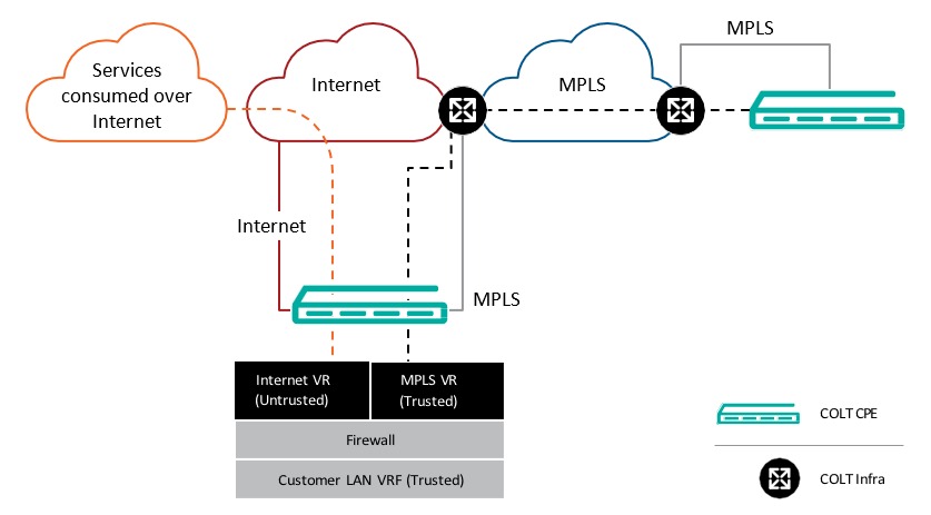
- Internet egress: Data leaving the cloud services for external destinations, where the provider bills for it.
- Internal transfers: Traffic between zones, regions or services, priced by route and service.
- Managed networking: Gateway availability, processed data, load balancers, public IP addresses and CDN operations, when deployed.
- Persistent data: Snapshots, backup retention, storage operations and retrieval fees for stored content.
VPC endpoints and alternative NAT designs change paths and costs, and they bring their own pricing and operational trade-offs. Whether they suit you is an architecture decision; the estimate needs to reflect the route you plan to deploy. If NAT gateways, VPC endpoints or egress traffic could change your decision, check the NAT Gateway traffic and charge diagnosis.
Include usage-based queries, functions, APIs and AI services
Individual operations create some of the biggest uncertainties. A serverless API can generate charges for invocations, execution time, database requests, logs and outgoing traffic. A reporting job can trigger repeated queries even when its application servers stay unchanged.
Google BigQuery is a specific example: under on-demand query pricing, billable data processing matters. Running the same report repeatedly raises the monthly number of bytes billed. Google’s documented maximum bytes billed setting rejects an on-demand query whose estimated chargeable bytes exceed the limit you set. An SQL LIMIT clause alone can leave the scanned bytes unchanged.
We recently got hit with a very large $19k+ unexpected Google Cloud BigQuery bill, and we’re trying to figure out what options we have. A single query pattern seems to have driven most of the charges, and the cost escalated far beyond what we expected. We are a startup, so this amount is a serious blow to our cash flow and could impact our ability to keep operating. We’ve already reached out to Google Cloud support, explained the situation, and asked for a waiver or credit, but so far we haven’t gotten a favorable outcome. We’re also trying to understand whether there are any other paths forward, such as escalation, payment arrangements, startup programs, or any way to get someone senior at Google to review the case.
The poster blames one query pattern, and the charge is an unverified personal account. The planning point still holds: when query volume is uncertain, put both the number of runs and the billable bytes per run in the estimate.
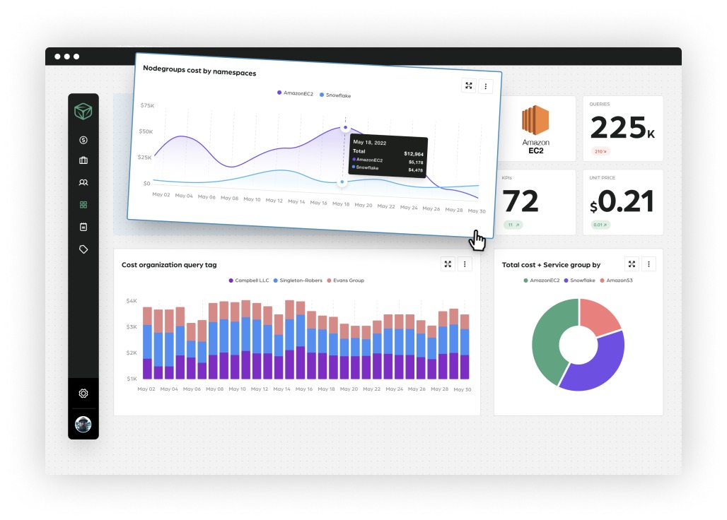
For one high-volatility feature, derive a monthly activity quantity from documented assumptions or application events: requests per day, reports per schedule, average query bytes, or input and output tokens by model. Include the storage, database and logging operations each event triggers when they carry metered charges.
Worked example: an itemized monthly cloud estimate
This is an illustrative teaching exercise with fictional unit prices, separate from AWS, Azure or Google Cloud price schedules. The example assumes two virtual machines running 730 hours in a month, a managed database, storage, outgoing traffic and NAT Gateway service charges. For AWS services, Azure regions, and Google Cloud networking, use the workload-based AWS, Azure, and Google Cloud comparison to compare requirements.
Multiply each quantity by its fictional rate and add the seven component subtotals.
| Component | Illustrative monthly quantity | Fictional rate | Fictional subtotal | Replace with live rate |
|---|---|---|---|---|
| Compute | 2 VMs × 730 hours | $0.10 per VM-hour | $146.00 | Provider SKU rate |
| Managed database | 730 instance-hours | $0.12 per hour | $87.60 | Provider DB rate |
| Attached block storage | 150 GB-month | $0.08 per GB-month | $12.00 | Storage class rate |
| Internet egress | 250 GB | $0.08 per GB | $20.00 | Relevant transfer rate |
| NAT Gateway availability | 730 gateway-hours | $0.04 per hour | $29.20 | Gateway hourly rate |
| NAT data processing | 300 GB | $0.04 per GB | $12.00 | Processed-data rate |
| Logs, backup and other services | Assumed fixed allowance | Fictional $18.00 allowance | $18.00 | Replace with individual SKUs |
| Total | $324.80 |
The two networking data quantities differ on purpose. Internet egress and NAT processing measure different paths or billable operations, and how they relate depends on the architecture, so copying one volume into both rows by default can distort the result.
The $18 allowance stands in for several meters; a real estimate itemizes them. The example also leaves out unlisted services such as a separately priced load balancer, additional replicas, public IPv4 addresses and cross-region replication. For decisions involving Savings Plans, Reserved Instances, and utilization coverage, see the Savings Plans versus Reserved Instances commitment analysis.
A workload without NAT drops those rows. One with additional replicas adds their compute, storage and traffic charges. Swap the invented quantities and prices for your configured services, calculate each line and check that the subtotals sum to the new monthly figure.
Low, expected and high scenarios for uncertain demand
A single estimate reflects one assumed pattern of use. To model uncertainty, change the quantities tied to plausible business events, such as a launch, seasonal traffic or a scheduled analytics job.
In the worked example, compute, database, storage, NAT availability and miscellaneous charges stay constant at $292.80. Only egress and NAT processed-data volumes vary, at the same fictional per-GB rates.
| Scenario | Internet egress | NAT processing | Fixed subtotal | Fictional monthly total |
|---|---|---|---|---|
| Low demand | 100 GB | 100 GB | $292.80 | $304.80 |
| Expected demand | 250 GB | 300 GB | $292.80 | $324.80 |
| High demand | 500 GB | 600 GB | $292.80 | $356.80 |
A workload that scales compute during a busy period needs variable compute rows too. A data-intensive report can change query cost without changing steady application capacity.
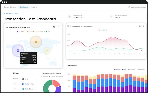
Every tool shows you a forecast of next month’s costs but they’re always wrong by like 30-40% which makes them basically useless for budget planning. They just extrapolate recent trends linearly which doesn’t account for seasonality, upcoming changes or any actual business context Q4 costs are always higher because holiday traffic, january costs drop because everyone’s on vacation but forecasts just see the december spike and predict january will be even higher. Then finance gets mad when actual costs are lower than the forecast and questions why the budget wasn’t fully used
The 30 to 40% figure is the contributor’s opinion, but the planning point stands: simple extrapolation of past spending misses business changes. FinOps forecasting ties observed spending to known usage drivers and planned operational events.
Cross-check the number with official pricing calculators
Provider calculators add service-specific configuration options and pricing bases. Build the same workload, with the same functional requirements, in each environment you compare.
- AWS: The AWS Pricing Calculator supports configured service estimates, regions and eligible pricing choices.
- Azure: The Azure Pricing Calculator accounts for service selection, region, usage and pricing agreements.
- Google Cloud: Its cost estimation guidance describes estimates built from specified configurations and anticipated usage.
A managed service can include responsibilities that another configuration requires you to provide separately. Compare compute capacity, database operations, redundancy and network paths when you evaluate configurations across providers.
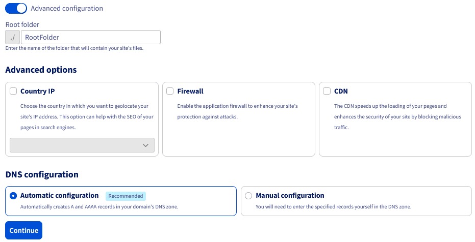
Save the calculated amount with its inputs: region, SKU, expected quantities, billing period, price source, price basis, currency and any discounts or credits. That lets you reproduce the estimate after rates or workloads change.
The Virginia Information Technologies Agency publishes cloud-cost scenarios using specific VM and disk configurations along with agency-specific chargeback adjustments. When you compare a provider subtotal with a chargeback amount, expect that extra accounting step.
Budget alerts, spending caps and enforcement limits

Monitoring a budget and enforcing a service limit are separate operations. A budget notification tells an owner about observed or forecast spending; an enforcement mechanism changes what future work the service accepts.
Azure Cost Management budget notifications leave underlying resources consuming services. Its documentation describes a cost-data delay, commonly 8 to 24 hours, so a threshold message can arrive after more charges accrue. AWS Budgets provides alerts and configured actions; scope, permissions, supported action types and billing-data timing govern their effect. Before changing cloud billing, cost allocation, or engineering owners, review the FinOps cloud-cost operating cycle for the implications.
Google Cloud also documents Preview spend-cap budgets for eligible services, including Gemini API, Gemini Enterprise Agent Platform, Cloud Run and Cloud Run functions. You configure a cap for one eligible service in one project. Its enforcement threshold uses gross estimated costs before discounts and credits.
When the threshold is reached, Google Cloud can pause eligible new usage. In-flight operations may still complete and incur charges, and enforcement can be delayed. Charges from persistent fixed resources, including compute or storage, fall outside the pause.
| Control | Purpose | Effect | Deciding condition |
|---|---|---|---|
| Azure budget notification | Warn of spending thresholds | Consumption continues | Billing-data and alert timing |
| AWS Budgets alert or configured action | Notify or trigger supported action | Depends on chosen action | Permissions, scope and data refresh |
| Google Cloud alert-only budget | Track estimated spend | Consumption continues | Monitoring and notification timing |
| Google Cloud Preview spend cap | Limit eligible service usage | Can pause new eligible work | Single service/project, delay, ongoing resources |
| BigQuery maximum bytes billed | Bound an on-demand query | Can reject an over-threshold query | Per-query usage guardrail |
The Google Cloud spend-cap documentation defines the Preview capability and its exclusions. A tokens-per-minute or requests-per-minute quota limits throughput, and its financial effect still depends on the allowed work and the billing meter.
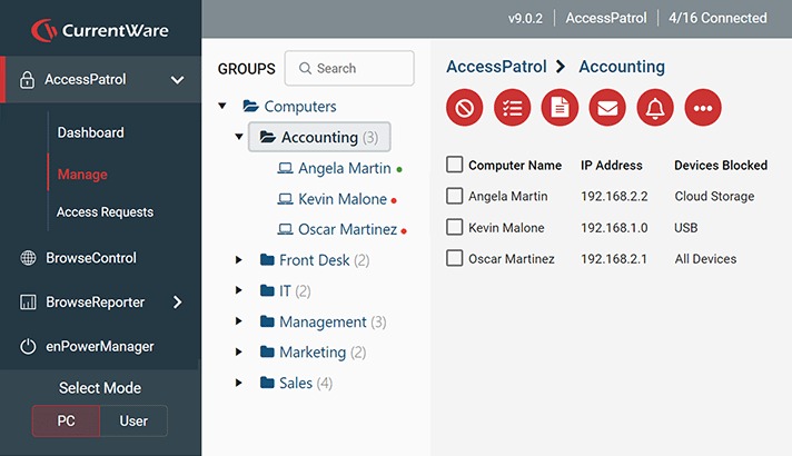
Classify each safeguard by the resource it governs, what triggers it, how quickly it is evaluated, and whether existing work can finish. A pause that protects a spending limit can also interrupt your application, so weigh availability requirements when you choose enforcement.
Reconcile the estimate with the real invoice

Your first bill lets you replace assumptions with observed usage. Compare estimated and billed quantities for the same service, meter, region, account and billing period, then examine the effective rate and any adjustments.
A variance can come from extra runtime, a larger stored volume, more expensive data paths, a new resource, a changed pricing tier or credit timing. Sorting the causes makes the next estimate more useful than writing off the whole difference as an overrun.
Our company’s AWS bill has been steadily climbing for the past few months and it’s starting to get out of control. We don’t even fully understand why. We have all the usual monitoring tools and dashboards, which tell us what services are costing the most (EC2, RDS, S3, of course), and when usage spikes. But things are still unpredictable. It feels like we’re constantly reacting. We see a spike, we investigate, maybe we find an obvious runaway process or an unoptimized query, we fix it, and then another cost center pops up somewhere else. It’s getting rly fkn annoying.
The account describes an ownership problem: EC2, RDS and S3 service totals are visible, while the responsible feature or engineering change stays hard to identify. AWS cost allocation tags help associate spending with resources and owners; user-defined tags must be activated to appear in billing reports.
Take the fictional NAT processing line again. If you estimated 300 GB and a hypothetical usage report recorded 400 GB, the difference is 100 GB. At the unchanged fictional $0.04 per GB, the line rises $4.00, from $12.00 to $16.00. Other line items stay constant in this illustration.
- Quantity difference: Compare expected and measured hours, GB, requests or query bytes.
- Rate difference: Compare the unit price you chose with the effective billed rate, including tiers and agreements.
- Resource or route difference: Find new services or changed network destinations.
- Billing adjustment: Find credits, timing changes and fee adjustments.
- Accountability: Tie the changed consumption to a deployment, environment or owner where possible.
Record estimated quantity and rate, actual quantity and rate, dollar delta, likely cause, owner and the revised assumption for the next period. Reporting delays, shared resources and later credits can limit how precisely you can attribute a charge to one feature.
Cloud bill versus full total cost of ownership
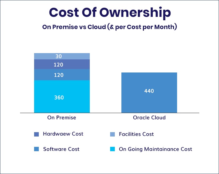
A cloud service estimate covers metered provider charges. Total cost of ownership also includes engineering labor, migration, support, licensing, training and compliance expenses over your chosen accounting period. Keep those organizational items in a separate budget column.
A forecast models future workload changes. Agency or reseller chargeback arrangements can add accounting terms beyond the provider subtotal.