
For steady, measurable request-unit demand, start by pricing provisioned throughput. For intermittent, single-region workloads with low total consumption, compare serverless. For variable traffic, weigh autoscale against its hourly peak-based charges. The right choice shifts with your measured usage, required regions, storage growth, and service limits. Check the resulting estimate against Azure Cost Analysis.
Which Azure Cosmos DB product and pricing model are you actually using?
Azure Cosmos DB has different pricing families. The first decision is whether you use an RU-based account or a vCore-based offering such as Azure Cosmos DB for MongoDB vCore. Their billing calculations use different units. This guide covers RU-based pricing, with Azure Cosmos DB for NoSQL as the main example. vCore needs a separate compute-and-storage calculation. Before you estimate anything, note your API, capacity mode, whether the account is new or existing, and your US deployment region in the Azure configuration. Then select the matching option on Microsoft’s Cosmos DB pricing page.
Manual throughput, autoscale, or serverless: which billing model fits?
Three apps can run the same number of database operations in a month and still get different bills. A consistently busy service, an occasional development environment, and an app with short traffic bursts each stress the billing model differently.
Provisioned throughput is measured in request units per second (RU/s). You pay for configured or billed throughput over time. Serverless charges for the request units (RUs) you consume plus storage, so the total amount of work drives the bill.
| Mode | Billing basis | Workload worth evaluating | Deciding constraint |
|---|---|---|---|
| Manual provisioned | Configured RU/s over billable hours | Predictable, sustained demand | Unused allocation remains billable |
| Autoscale provisioned | Highest scaled RU/s within each hour, subject to the minimum | Traffic that rises and falls | Hourly peaks, configured Tmax, and capacity floor |
| Serverless | RUs consumed and stored data | Intermittent, relatively low-consumption demand | Single-region deployment and applicable service limits |
Manual throughput is the simplest to account for. The level you set keeps incurring its charge during quiet periods, which suits an app whose sustained demand uses much of the reserved capacity.
With standard autoscale, you set a maximum throughput, or Tmax. The account scales between 10% of Tmax and the maximum. Billing follows the highest throughput reached in an hour, even if that peak lasted only part of it.
For a single-write-region account, the autoscale rate per 100 RU/s-hour is 1.5 times the manual provisioned rate. The multiplier applies to the hourly unit rate, and your monthly charge follows the capacity billed in each hour. Multiwrite-region pricing follows different rules.
With dynamic autoscale, throughput scales independently across physical partitions and regions, which changes how billed capacity is aggregated. Base your estimate on the autoscale configuration your account uses.
Serverless removes the need to allocate RU/s in advance. It suits a lightly used app with long idle periods, provided the workload fits the capacity mode. Microsoft’s capacity-mode comparison limits serverless to a single region.
Eligible provisioned resources can switch between manual and autoscale throughput. Moving an existing provisioned account to serverless may require creating another account and migrating data.
One operator ran into that limit as the workload changed:
One of my biggest issue with cosmosdb is that I cannot change from provisioned to serverless. Usage of containers changes over the lifecycle of product and i am stuck with multiple accounts which are provisioned and it makes more sense to be serverless for cost. Also why cannot i provision less that 400 RU in manual or 1000 in autoscale.
How many request units does your application really use?
The RU charge of each operation is the number to measure when you estimate Cosmos DB consumption. Operations differ in the work they do, the data they touch, and the partitions they reach.
An RU is the normalized cost of one operation. RU/s is capacity or demand per second. Total monthly RUs are the work done over the billing period. Serverless bills the monthly total. Provisioned throughput bills RU/s.
Microsoft’s request-unit documentation gives a reference point: reading a 1-KB item by its ID and partition key costs about 1 RU.
A query that scans more data, a write that maintains indexes, and a targeted point read can generate very different request charges. Item size, indexing policy, query design, partition targeting, and consistency settings all change the amount of work.
Build a representative workload record
| Input | Measure | Evidence | Use in the estimate |
|---|---|---|---|
| Operation mix | Reads, writes, queries | Application request logs | Separate operations with different RU costs |
| Request charge | RU per operation | x-ms-request-charge or SDK diagnostics | Calculate consumed RUs |
| Request counts | Operations during the billing period | Application telemetry | Scale sampled request charges to workload totals |
| Peak throughput | RU/s by time interval | Application and Azure metrics | Size capacity and characterize bursts |
| Throttling | 429 responses and normalized utilization | Service diagnostics | Identify capacity pressure |
| Partition use | Demand across partition keys | Partition-level diagnostics | Identify uneven workload distribution |
The request-charge header gives you an observed RU value for each operation. Sum representative charges across your real operation mix to estimate consumption. The timing of those operations shows the peaks a provisioned account has to handle.
A developer running a small MERN registration app reported that database operations failed at 400 RU/s and worked at 2,000 RU/s:
I’m currently using Cosmos DB in my MERN stack application. When I set the Request Units (RU/s) to 400, the database operations fail or don’t respond properly. However, when I increase the RU value to 2000, everything works as expected — even though the website is relatively small and only handles basic user registration (name, email, phone number, password, and confirm password). Since Cosmos DB charges increase significantly with higher RU values, this is becoming costly. I’m trying to understand why such a simple operation is requiring 2000 RU/s, and how I can optimize or resolve this to reduce the cost.
The cause of the trouble at 400 RU/s is unresolved. HTTP 429 responses, cross-partition queries, uneven partition demand, and retry behavior would each point to a different diagnosis. Request-charge traces and partition metrics show what demand sits behind the registration form.
Capture request charges and response diagnostics during both ordinary and busy periods. Compare them with normalized throughput utilization, partition demand, and throttling events.
Why can indexing, partitions, and data growth raise the bill?

Cosmos DB costs can stay high after traffic drops, because operation efficiency and minimum configurable capacity are separate cost mechanisms.
Indexing affects the work done when documents are written and how queries retrieve data. Maintaining indexes can raise write charges. Index data also takes up storage, and unsuitable query and indexing choices can consume more RUs on reads.
One contributor saw query charges fall sharply after an indexing change:
For me the main issue with the cost is that the indexing configuration is a bit of a dark art. We had a cosmos database that was wildly inefficient until one of my colleagues sorted out the indexing and the RU cost per query went down to literally less than 1% of the original cost. I think this part should be more intuitive. Architecturally cosmos is a great option. Managed nosql that is lightning fast! But operationally it can be a pain to wrangle.
Partition distribution is a separate problem. If one partition key takes much of the traffic, some physical partitions come under pressure while other capacity sits mostly idle. Raising the total allocation can leave the uneven distribution unresolved.
Minimum configurable Tmax and stored data
For a dedicated autoscale container, Microsoft’s minimum maximum-throughput calculation when you reduce Tmax has three constraints:
- Baseline: 1,000 RU/s.
- Historical capacity: One-tenth of the highest Tmax previously provisioned.
- Storage: Stored GB multiplied by 10 RU/s per GB.
The dedicated-container expression is:
Minimum configurable Tmax = MAX(1,000 RU/s, highest-ever Tmax / 10, stored GB × 10 RU/s)
The result is subject to rounding and supported throughput increments. New shared-throughput databases are generally subject to Microsoft’s 25-shared-container limit; eligible existing databases and subscriptions may have exemptions. For an eligible shared-throughput database with more than 25 shared containers, the minimum calculation also includes 1,000 + MAX(container count - 25, 0) × 1,000 RU/s among the limiting terms.
This minimum is the maximum throughput the resource can be set to after a reduction. The instantaneous autoscale floor, the 10% of Tmax described earlier, is a different limit.
Storage growth can raise the minimum configurable maximum even while request traffic falls. A historically high Tmax does the same. A quiet monitoring period alone does not mean you can lower a throughput setting.
What else appears on an Azure Cosmos DB bill besides throughput?
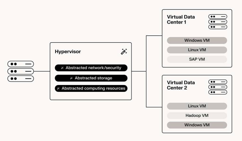
Throughput or consumed RUs are only one billing category. Storage, replicated regions, backup choices, and enabled features can raise the total even when your traffic stays the same. An account replicated to several regions incurs throughput and storage charges across its deployment topology.
| Cost component | What creates the charge | Configuration that matters |
|---|---|---|
| Throughput or request consumption | Provisioned RU/s over time or consumed RUs | Capacity mode, allocation, workload |
| Transactional storage | Item and index data | Stored GB, indexing, regions |
| Replicated capacity | Capacity across deployment regions | Region count and write topology |
| Backup and restore | Applicable backup or restore meters | Backup mode and recovery features |
| Analytical storage | Additional storage where enabled | Analytical features and data volume |
| Network and other meters | Applicable bandwidth, availability, or service-specific charges | Architecture and enabled options |
Multi-region reads and writes can change the quantity and pricing of provisioned capacity, as well as the amount of replicated storage.
A complete worksheet follows this structure:
Estimated total = throughput or RU charges + storage + applicable additional meters - eligible allowances and discounts
What would two different Cosmos DB workloads cost?
Microsoft’s published examples show how total monthly request consumption can change serverless’s advantage over manual provisioned throughput.
The manual example is 500 RU/s for 730 hours at a published example rate of $0.008 per 100 RU/s-hour. Five 100-RU/s units over 730 hours give a throughput subtotal of $29.20.
| Published example | Manual provisioned subtotal | Serverless RU subtotal | Important qualification |
|---|---|---|---|
| 500 RU/s for 730 hours | $29.20 | Depends on consumed RUs | Throughput only; storage excluded |
| 20 million consumed RUs | $29.20 | $5.00 | Uses the same illustrative 500 RU/s capacity assumption |
| 250 million consumed RUs | $29.20 | $62.50 | Uses the same illustrative 500 RU/s capacity assumption |
The manual calculation is $0.008 × (500 / 100) × 730 = $29.20. Serverless uses the example rate of $0.25 per million RUs, so its subtotal moves with the monthly amount of work.
These rates come from Microsoft’s published examples. Use the rates for your US region when you estimate a deployment. The 500 RU/s assumption holds only for a workload whose peaks and partition demands fit that capacity.
Build an estimate for each billing mode
Manual provisioned throughput starts with configured capacity, billed hours, regions, and the current hourly price:
Manual throughput subtotal = SUM((billable RU/s / 100) × regional price per 100 RU/s-hour, across billed hours and regions)
Provisioned-throughput billing follows Microsoft’s wall-clock-hour rules. A resource created and deleted within five minutes still incurs a full hour’s charge. Throughput changes within an hour follow the documented billing method.
For serverless, the request subtotal follows your measured workload:
Serverless RU subtotal = (monthly consumed RUs / 1,000,000) × regional price per million RUs
Autoscale needs an hourly capacity profile. Use Azure Monitor to check the configured autoscale maximum RU/s and the throughput the resource scaled to during each hour. For standard autoscale, the highest scaled capacity reached in each billing hour, subject to the minimum, is the billable capacity:
Autoscale subtotal = SUM((hourly billable RU/s / 100) × applicable autoscale price per 100 RU/s-hour)
For example, 6,000 RU/s is 60 units of 100 RU/s. At 1.5 times the manual rate, that hour costs the same as 90 manual units. For compute hours, storage usage, and network egress, use the cloud cost estimation worksheet to compare the relevant requirements.
Dynamic autoscale also requires its documented region and physical-partition billing aggregation, so an account using it needs the corresponding observed capacity values.
Reproduce Microsoft’s examples in a worksheet. Then swap in your actual monthly RUs, required capacity, and hourly peak distribution, and add the storage and other charges that apply to your deployment.
Can free tier or discounts change the answer?
An eligible Azure Cosmos DB account can receive a dedicated free-tier allocation. Microsoft’s free-tier documentation specifies 1,000 RU/s and 25 GB, subject to eligibility and account-level conditions.
You opt in when you create an eligible account, and the allowance applies to at most one qualifying Cosmos DB account per Azure subscription. It applies to eligible provisioned-throughput configurations. Serverless accounts do not receive the dedicated free-tier allocation.
This benefit is separate from time-limited offers tied to an Azure free account. The two have different eligibility requirements.

Additional regions, storage above the allowance, or separately billed features can still produce charges on a qualifying account.
Reserved capacity and other eligible commercial discounts can also affect provisioned-throughput cost. Their value depends on the offer, commitment terms, region, and subscription pricing.
Why does the Azure Cosmos DB bill differ from the estimate?
Your bill reflects the meters and the capacity or consumption recorded for the billing period, so compare like with like: the same account, region, billing period, and charge category. A mismatch in any of those can make a correct calculation look wrong.
Reconcile the forecast with the invoice
- Open the cost breakdown. In the Azure portal, choose the subscription or supported billing scope, open Cost Management and Cost Analysis, and filter Service name to Azure Cosmos DB. Group or export charges by meter, region, and scope. Access depends on your billing permissions.
- Compare provisioned capacity. For manual throughput, match configured RU/s and billable hours. For autoscale, compare billed hourly capacity with the maximums reached and the minimum. Account for dynamic autoscale aggregation where enabled.
- Compare workload measurements. Check request-charge telemetry, observed RU/s demand, normalized utilization, and any 429 responses. Did your forecast capture peak demand and uneven partition activity?
- Match additional meters. Match transactional storage, index storage, regional replicas, backup, and other enabled features to the corresponding lines in your estimate.
- Apply commercial terms. Compare free-tier allocations, reservations, and subscription discounts with the charges in question.
- Isolate unexplained differences. Calculate the remaining variance by meter and keep unidentified charges for account-specific billing investigation.

Microsoft announced the Azure Cosmos DB Cost Estimator for NoSQL in public preview in June 2026. The announcement described workload-based projections and configuration comparisons that can inform estimates before a deployment is configured.
The estimator’s projections rest on its stated pricing and configuration assumptions. Negotiated subscription terms, service constraints, and the final deployment can change your bill.
A higher-than-expected charge may come from extra billable throughput hours, a different hourly autoscale profile, storage growth, regional replication, or a discount that did not apply. The checks for cloud billing, cost allocation, and engineering owners are explained in the FinOps cloud-cost operating cycle.
Which Cosmos DB pricing approach makes sense for your workload?
Database design decides whether a capacity mode delivers the performance you expect for the price. Partition distribution, query efficiency, and data-model choices all change how well your app uses provisioned capacity or consumed RUs.
One team running large production systems described the trade-off of denormalizing:
Been using for about 4 years. Massive production systems for multiple customers. For our use case it is incredible and means we’re serving millions of API requests with performance SLAs our competitors could only dream about. To pull that off we had to denormalise in a few places, little bit more work on coordinating updates. We migrated around 20 million records into the system. No issues, stayed snappy, all done over a weekend (not solid imports, just the allocated period). I like it because it’s conceptually simple so everyone can design with it and not need to know bucket loads about it under the covers.
Denormalizing can simplify retrieval while requiring extra coordination of updates. Both affect RU use and operational complexity.
Use your completed cost comparison to pick a configuration, and decide in advance when you will revisit it.